

A Reinforcement Learning header-only template library for C++14. Minimal and simple to use, for a variety of scenarios. It is based on Sutton and Barto’s book [1] and implements some of the functionality described in it.
Currently the library implements the following algorithms, each one explained in its own document (with the formulas, the pseudocode, and how to use it):
- Q-Learning (
q_learning) for deterministic systems, as well as non-deterministic systems (q_probabilistic), see docs/q_learning.md - SARSA (
sarsa) and Expected SARSA (expected_sarsa), which learn the value of the policy the agent actually follows, exploration included, see docs/sarsa.md - Double Q-Learning (
double_q_learning), which keeps two estimates, so that the one picking the best next action is not the one valuing it, and isn’t fooled by noisy values, see docs/double_q_learning.md - Dyna-Q and Dyna-Q+ (
dyna_q), which remember every move made, and replay them in their head (planning) to learn far more from the same experience, whilst Dyna-Q+ also goes back to check moves it hasn’t made for a while, in case the world has changed, see docs/dyna.md - Monte Carlo control (
monte_carloandoff_policy_monte_carlo), which waits for each episode to end, and learns from the rewards that actually followed, with exploring starts, on-policy (ε-Greedy), or off-policy with importance sampling, see docs/monte_carlo.md - off-policy Monte Carlo prediction (
off_policy_monte_carlo_prediction), which learns the values of any policy from episodes played by another, with ordinary, weighted, discounting-aware or per-decision importance sampling, see docs/monte_carlo.md - Monte Carlo Tree Search (
mcts), with UCT, which plans each move as it is about to make it: it plays thousands of games in its head with a model of the game, spending more of them on the moves that look best, and supports two players (each value from the point of view of the player who moved), see docs/mcts.md - TD(0) and n-step TD prediction (
n_step_td), and n-step SARSA (n_step_sarsa), which learn from the next n rewards and then the value of the state reached, anywhere between one-step TD and Monte Carlo, see docs/n_step.md - n-step Expected SARSA (
n_step_expected_sarsa), off-policy n-step SARSA (off_policy_n_step_sarsa), the tree backup algorithm (n_step_tree_backup) and Q(σ) (n_step_q_sigma), which learn n steps at a time, on-policy or off-policy (the values of a greedy policy from an agent that explores), with or without importance sampling, see docs/n_step.md - TD(λ) (
td_lambda), SARSA(λ) (sarsa_lambda) and Watkins’s Q(λ) (watkins_q_lambda), whose eligibility traces share every TD error with the moves that led to it, accumulating or replacing, see docs/eligibility_traces.md - true online TD(λ) (
true_online_td_lambda) and true online Sarsa(λ) (true_online_sarsa_lambda), which learn after every step with Dutch traces, and have after every step exactly the values of the online λ-return algorithm, see docs/eligibility_traces.md - REINFORCE, REINFORCE with a baseline and one-step Actor-Critic (
reinforce,reinforce_with_baselineandactor_critic), which learn the policy itself, as a softmax over action preferences (softmax_policy), so that it can stay stochastic when that is best, see docs/policy_gradient.md - Actor-Critic with eligibility traces (
actor_critic_lambda), whose critic shares each TD error with the states visited before and whose actor with the actions taken before, and Actor-Critic for tasks that never end (continuing_actor_critic), which learns the average reward per step, see docs/policy_gradient.md - R-Learning (
r_learning) and differential Sarsa (differential_sarsa), for tasks that never end: they learn the average reward per step, and how much better than average each action is, after every step, see docs/r_learning.md - Prioritized sweeping (
prioritized_sweeping), which plans like Dyna-Q, but replays first the moves whose values would change the most, working backwards from every change, see docs/prioritized_sweeping.md - Dynamic programming (
dynamic_programming, with a modelfinite_mdp): policy evaluation, policy iteration and value iteration, which need no playing at all when the rules of the world are known exactly, see docs/dynamic_programming.md - UCB (
ucb) and the gradient bandit (gradient_bandit), for the k-armed bandit: UCB explores the arms it is least sure about, whilst the gradient bandit learns a preference for each arm, and picks arms with their softmax, see docs/bandits.md - schedules for the learning rate and the exploration rate, so that each one can decay as the agent learns
(
polynomial_decay,exponential_decayandlinear_decay), see docs/schedules.md. Do bear in mind thatq_learning,sarsa,expected_sarsa,double_q_learningand the n-step learners can each decay the learning rate of every state/action pair on its own
It also comes with a collection of classic games to learn, described in Games below.
Implementation in C++
The template class policy stores the learnt values of your states and actions.
A pair of template wrapper classes, state and action, is provided in the header, which wrap around your own
state and action structures (the state_trait and action_trait). Those can be anything, provided that:
- they have an
operator== - they are hashable, with a specialisation of
std::hash
Take care to make them unique, two different states whose traits compare equal are treated as one.
The examples/gridworld_header.hpp shows how to write them.
You can also create your own state and action classes and use them instead of the wrappers,
but they must satisfy the below criteria:
- they have an
operator== - they have a specialisation of
relearn::hasher - states must expose their reward with a method
reward()
Markov Decision Process
An MDP is a sequence of States st linked together by actions at.
At the core of relearn is the policy which uses MDPs and maps them using the rewards R received along them.
Whilst multiple episodes may exist, and an episode may be iterated many times, updated, evaluated
and re-experienced, the actual process is done in class policy. An overview of an MDP is shown below.
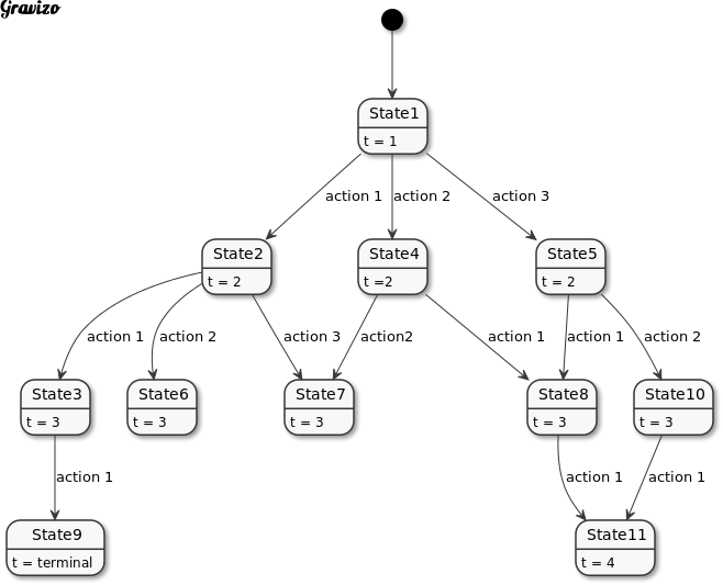
The template parameters state_trait and action_trait are used to describe what a state and action are,
the wrappers are used only for indexing, hashing and policy calculation.
The basic use is to create episodes, denoted as markov_chain which you populate as you see fit,
giving each step the reward it earned (any value, positive, negative or zero).
Do bear in mind that each reward belongs to the step that earned it, have a look at the
reward convention.
The use of a markov_chain defaults to an std::deque<relearn::link<state_class,action_class>>
where relearn::link is the struct encapsulating a state/action observation.
You may replace the container or link class if you want, but the learners require that:
- the episode has an
operator[]taking the index of a link, and asize()method - each link has the members
stateandaction
Basically std::deque and std::vector work right out of the box (std::list won’t, as it has no operator[]).
The library uses by default double for storing and updating Q values,
but you can play around with it if needed.
The class that mostly interests us is policy which uses your states and actions,
and stores them in a map of states, where each state (key) has a value of maps (action to value):
.
├── s_t
|   ├── a_t: 0.03
|   └── a_t: -0.05
├── s_t
|   ├── a_t: -0.001
|   └── a_t: 0.9
You own and control the policy objects, and you can even use multiple ones, however bear in mind that they are not locked for MT access (you have to do this manually). Using any of the learners you can then set/update the policy values by iterating your episodes.
Dependencies
There are no external dependencies! However, your compiler must support C++14, so you will need:
- GCC 5 or higher
- Clang 3.4 or higher
These are the first releases with complete C++14 support. The CI builds with GCC on Ubuntu, and with Apple Clang on macOS.
note: I haven’t tested with a Windows platform!
note: building the examples and tests needs CMake 3.5 or higher, and the tests use Catch2 v2, whose single header is downloaded by CMake.
note: serialization is optional, and needs Boost (see enable serialization below).
Building
There is nothing to build! This is a header-only library, you only need the src folder, and to include the relearn.hpp header.
However, you may compile the examples in order to see how the library is used.
relearn.hpp simply includes the parts of the library, which live in src/relearn/, one header for each:
| header | what’s in it |
|---|---|
relearn/core.hpp |
state, action, the link of an episode, and the policy |
relearn/schedules.hpp |
polynomial_decay, exponential_decay, linear_decay, and the visit_counter |
relearn/q_learning.hpp |
q_learning and q_probabilistic |
relearn/sarsa.hpp |
sarsa and expected_sarsa |
relearn/double_q_learning.hpp |
double_q_learning |
relearn/dyna.hpp |
dyna_q |
relearn/monte_carlo.hpp |
monte_carlo and off_policy_monte_carlo; off_policy_monte_carlo_prediction |
relearn/mcts.hpp |
mcts, Monte Carlo Tree Search with UCT |
relearn/n_step.hpp |
n_step_sarsa, and n_step_td (TD(0) when n = 1); n_step_expected_sarsa, off_policy_n_step_sarsa, n_step_tree_backup and n_step_q_sigma |
relearn/eligibility_traces.hpp |
sarsa_lambda, td_lambda and watkins_q_lambda, and their eligibility_traces; true_online_sarsa_lambda and true_online_td_lambda |
relearn/policy_gradient.hpp |
softmax_policy, reinforce, reinforce_with_baseline and actor_critic; actor_critic_lambda and continuing_actor_critic |
relearn/r_learning.hpp |
r_learning and differential_sarsa |
relearn/prioritized_sweeping.hpp |
prioritized_sweeping |
relearn/dynamic_programming.hpp |
finite_mdp and dynamic_programming |
relearn/bandits.hpp |
ucb and gradient_bandit |
Each one includes whatever it needs, so if you only use one learner (e.g., on a small board, where every byte
and every second of compiling counts) feel free to include just that one, #include "relearn/q_learning.hpp".
To do that, simply:
mkdir build
cd build
cmake ..
make
This builds all the examples, as ex_<name> in the build folder.
build tests
cmake .. -DBUILD_TESTS=On
make
ctest
enable serialization
In order to enable serialization, you need boost and boost-serialization. See your distro on how to install those. To enable it, pass a cmake flag:
cmake .. -DUSING_BOOST_SERIALIZATION=On
For example if you want to run the tests with serialization:
cmake .. -DUSING_BOOST_SERIALIZATION=On -DBUILD_TESTS=On
You can also use serialization in your own project, if you wish to save and load
policies, states or actions: simply define USING_BOOST_SERIALIZATION (e.g., -DUSING_BOOST_SERIALIZATION)
before including relearn.hpp, and use CMake’s find_package to find, include and link against boost_serialization.
Do bear in mind that the state_trait (e.g., your state descriptor) and the
action_trait (e.g., your action descriptor) must also be serializable.
On how to achieve this, have a look at this tutorial
if this condition is not met, you will end up with compilation errors.
Because of the flexibility of boost serialization, you can save and load binary, text or xml archives.
Later versions of boost support smart pointers, so even if your descriptors are
std::shared_ptr or std::unique_ptr you can still save and load them.
Examples
There is a folder examples with two “Gridworld” examples:
- an offline one, which learns from random exploration:
examples/gridworld_offline.cppbuilt asex_gridworld_offline - an online one, which learns after every episode:
examples/gridworld_online.cppbuilt asex_gridworld_online
and a collection of classic games, described in Games below.
basic usage
The basic way of using the library is the following:
- create a class state, or use an existing class, structure, or POD which describes (in a Markovian sense) your state
- create a class action, or use an existing class, structure, or POD which describes the action.
- create an episode which by default is an
std::deque<relearn::link<state,action>>, and populate it with the steps taken and the reward each one earned.
At this point, depending on whether you are using an online or offline algorithm/approach, you have the following options:
- keep creating episodes, and once you have finished, train the policy with all of them, or
- every time you create an episode, train your policy with it.
That choice is up to you, and almost always depends on the domain, system or problem you’re trying to solve.
It is for this reason that there is no implementation of on_policy or off_policy or e_greedy,
those are very simple algorithms, and are application-specific.
The games show one way of writing them (games::greedy and games::epsilon_greedy in examples/games/game.hpp).
UCB and the gradient bandit, on the other hand, are whole algorithms for bandits, so they are in the library
(have a look at docs/bandits.md).
Take a look at the gridworld examples, which demonstrate two different ways of achieving the same task.
The blackjack example is different: Blackjack is a game of chance, where the same decision can win or lose
depending on the cards that follow, so it uses q_probabilistic, which learns the expected reward and the
probability of each transition from the games it plays.
The blackjack_monte_carlo example learns the same game with Monte Carlo instead, in three different ways.
The tic_tac_toe_mcts example does not learn at all: it plans every move with Monte Carlo Tree Search,
using a model of the game (examples/games/tic_tac_toe_model.hpp).
Gridworld
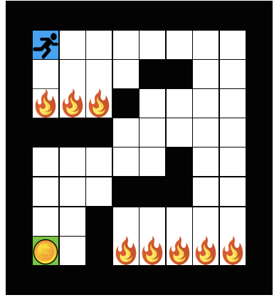
The pinnacle of simplicity when it comes to block/grid world toy problems, our agent resides in a 10x10 gridworld, which is surrounded by blocks into which it can’t move (black colour). The agent starts at blue (x:1,y:8) and the target is the green (x:1,y:1). The red blocks are fire/danger/a negative reward, and there is a rudimentary maze. Moving into the target earns +1, moving into a fire block earns -1, and both end the episode.
Both versions learn with Q-Learning, which learns the values of the best actions, whatever actions were taken whilst exploring. They differ in how they explore. The offline approach:
- first the agent randomly explores until it can find the positive reward (+1.0) grid block
- then it updates its policies
- finally it follows the best policy learnt
And the online approach:
- the agent explores one episode
- then it updates its policies
- then it tries again, this time following the policies it knows
- it only falls back to random when there does not exist a positive best action (or it leads into a wall)
- the entire process is repeated until the goal is discovered.
The actual gridworld is saved in a textfile examples/gridworld.txt (feel free to change it).
The header examples/gridworld_header.hpp provides the minimal code to demonstrate this staged approach.
The two files:
examples/gridworld_offline.cppexamples/gridworld_online.cpp
have the different versions of how this task can be solved.
Once we have loaded the world (using function populate) we set the start at x:1, y:8 and then
begin the exploration.
offline q-learning
The offline exploration runs in an infinite loop until the grid block with a positive reward is found.
Until that happens, the agent takes a stochastic (e.g., random) approach and searches the gridworld.
The function (template parameter S is state, and A is action):
template <typename S,
          typename A>
std::deque<relearn::link<S,A>> explore(const world & w,
                                       std::mt19937 & gen,
                                       grid start);
does the following:
- creates a new episode (e.g.,
relearn::markov_chain) - starts from the starting gridblock
- randomly picks a direction (see struct
rand_directionfor more) - records each step with the reward of the block it moved into
- repeats this until either (a) a negative reward has been found (e.g., stepped into a fire block), or (b) the goal block is discovered
Each time the explore method is called in the main exploration loop,
an episode is acquired, which is then appended in the list of experienced episodes std::vector<std::deque<relearn::link<state,action>>> episodes.
Once the agent has found the target gridblock, it updates its policy memory using those episodes:
auto learner = relearn::q_learning<state,action>{0.9, 0.9};
for (int k = 0; k < 200; k++) {
    for (const auto & episode : episodes) {
        learner(episode, policies);
    }
}
In this instance, the agent will run two hundred iterations for each episode, since each pass moves the reward only one step back towards the start, and random episodes can be long. The actual Q-Learning parameters are:
- alpha (learning rate) 0.9
- gamma (discount) 0.9
Finally, once updating policies has finished, the agent proceeds to follow (once) the best action policy:
on_policy(w, policies, start);
The result is that the agent will go straight from x:1, y:8 to x:1, y:1 avoiding any fire blocks and unnecessarily searching the gridworld.
This is a deterministic scenario, because the agent knows at any given moment, which action it is taking, and to which state that action will lead to.
online q-learning
The online exploration is somewhat different, because the explore method does the following:
- creates a new episode
- starts from the starting gridblock
- if a good policy (a Q value higher than zero, for a move that does not lead into a wall) exists, it follows it
- else if no good policy exists, it takes a random action
- repeats until a reward is found, it then trains the policies with the latest episode (ten passes)
- an episode that wanders for more than 1000 moves is cut short, and learnt with
terminated = false(see episodes cut short), so that its last move is not learnt as the end of the game
The difference here, is that the actual exploration is instantly affected by what has already been learnt. In comparison, the offline method is not affected, and may repeat the same sequences over and over again. However, if the online version stops too early, there is no guarantee that the agent has learnt the ideal or optimal path to the goal, it could in fact be just a mediocre or silly path it has discovered. This of course, is also a problem with offline, where the solution may never be discovered.
Other approaches exist (e.g., ε-Greedy) where the agent may follow the policy, but randomly choose to ignore it, in order to try and discover a better solution. The games below use ε-Greedy.
Games
The folder examples/games holds classic reinforcement learning problems, each one in its own header,
and examples/<game>.cpp learns each one (built as ex_<game>). Most of them come from Sutton and Barto [1],
whereas FrozenLake, cart-pole and mountain car follow Gymnasium’s [2] rules and physics, so that agents can later be
compared on both.
Every game has the same shape, after Gymnasium’s reset()/step() (see examples/games/game.hpp):
games::cliff_walking game;
auto s = game.reset();                        // start an episode
auto out = game.step(games::right);           // out.next, out.reward, out.terminated
auto moves = game.actions(s);                 // the legal actions
and games::play records an episode in relearn’s reward convention, ready for a learner:
using types = games::types<games::cliff_walking>;
types::policy memory;
relearn::q_learning<types::state, types::action> learner;
auto r = games::play(game, [&](const auto & s, const auto & legal) {
    return games::epsilon_greedy<games::cliff_walking>(memory, s, legal, 0.1, prng);
}, 1000);                                     // at most 1000 moves
learner(r.episode, memory, r.terminated);     // a cut-short episode is not learnt as finished
Alternatively, games::play_online plays an episode and learns after every step, as Sutton and Barto’s
TD algorithms do. SARSA needs it with a large learning rate (have a look at docs/sarsa.md):
auto r = games::play_online(game, agent, learner, memory, 1000);
The n-step learners need the last n steps after each step, not just the last one, so give play_online their n:
games::play_online(game, agent, learner, memory, 1000, learner.n) (have a look at docs/n_step.md).
The learners with eligibility traces learn a whole episode at a time, so use games::play with them; all but
true_online_sarsa_lambda and true_online_td_lambda, which learn after every step with games::play_online.
| Game | Source | Learnt with | What it shows |
|---|---|---|---|
bandit |
S&B 2.3 | q_probabilistic |
Exploration vs exploitation, greedy vs ε-Greedy (Figure 2.2) |
bandit_ucb_gradient |
S&B 2.7, 2.8 | ucb, gradient_bandit |
UCB earns more than ε-Greedy (Figure 2.4), and the gradient bandit needs its baseline (Figure 2.5) |
blackjack |
S&B 5.1 | q_probabilistic |
A random game, where the learnt strategy matches Figure 5.2 |
blackjack_monte_carlo |
S&B 5.3, 5.4, 5.7 | monte_carlo, off_policy_monte_carlo |
The same game learnt from whole games: with exploring starts, on-policy, and off-policy from games played at random |
importance_sampling |
S&B 5.5 to 5.9 | off_policy_monte_carlo_prediction |
The value of a policy learnt from another’s play: ordinary against weighted importance sampling on a blackjack state (Figure 5.3), an infinite variance (Example 5.5), and discounting-aware and per-decision importance sampling on long episodes |
cliff_walking |
S&B 6.6 | q_learning, sarsa, expected_sarsa |
On-policy vs off-policy: Q-Learning learns the path along the cliff edge, SARSA a safer one, and both SARSAs earn more whilst exploring |
windy_gridworld |
S&B 6.5, Ex. 6.10 | both Q-Learnings | Steady wind: the 15-move path. Random wind: q_probabilistic, and q_learning with a learning rate that decays per pair, find the best policy, whereas q_learning with α = 0.5 does not |
random_walk |
S&B 6.2, 7.1 | q_probabilistic |
Prediction, with the learnt values next to the exact ones |
random_walk_td |
S&B 6.2, 7.1 | n_step_td, monte_carlo |
TD(0) learns faster than Monte Carlo (Example 6.2), and an intermediate n is best (Figure 7.2) |
random_walk_lambda |
S&B 12.1, 12.2, 12.5 | td_lambda, true_online_td_lambda |
An intermediate λ is best (Figure 12.6), offline TD(λ) learns exactly what the λ-return does, and true online TD(λ) learns at least as well as TD(λ), without blowing up at a large α |
maximization_bias |
S&B 6.7 | q_learning, double_q_learning |
Q-Learning’s overestimation, which Double Q-Learning removes (Figure 6.5) |
gamblers_problem |
S&B 4.3 | q_probabilistic |
Values that match the exact solution |
dynamic_programming |
S&B 4.1, 4.3, 4.4 | dynamic_programming |
The 4 x 4 gridworld (small_gridworld, Figure 4.1) and the gambler’s problem (Figure 4.3) solved from their models, by policy evaluation, policy iteration and value iteration |
dyna_maze |
S&B 8.1 to 8.3 | dyna_q |
Planning learns a maze in far fewer episodes (Figure 8.2), and Dyna-Q+ copes with mazes that change (Figures 8.4, 8.5) |
dyna_maze_n_step |
S&B 7.2, 8.1 | n_step_sarsa |
The first episode teaches n-step SARSA its last n moves (Figure 7.4), so a larger n learns the maze faster |
cliff_walking_n_step |
S&B 6.6, 7.2 to 7.6 | n_step_expected_sarsa, off_policy_n_step_sarsa, n_step_tree_backup, n_step_q_sigma |
Learning 4 steps at a time: on-policy, the expectations earn more whilst exploring; off-policy, the less importance sampling, the closer to the greedy policy’s values |
dyna_maze_lambda |
S&B 12.7, 12.10 | sarsa_lambda, watkins_q_lambda |
With replacing traces, one episode is enough to find the goal again; accumulating traces get lost in the loops |
mountain_car_lambda |
S&B 10.1, 12.7 | true_online_sarsa_lambda |
Learning after every step: from the second episode on, the longer the traces, the fewer steps to the flag, little more than half of SARSA’s with λ = 0.95 |
short_corridor |
S&B 13.1 | reinforce, reinforce_with_baseline, actor_critic, actor_critic_lambda |
Cells that look the same, where the best policy is stochastic: REINFORCE learns it (Figure 13.1), faster with a baseline (Figure 13.2), whereas one-step Actor-Critic’s critic misleads it, and Actor-Critic with traces learns it best |
access_control |
S&B 1st ed. 6.7, 2nd ed. 10.2, 13.6 | r_learning, differential_sarsa, continuing_actor_critic |
A task that never ends: accept or reject customers to earn the most per step, against the exact optimal policy (Figures 6.17, 10.5) |
dyna_maze_prioritized |
S&B 8.4 | prioritized_sweeping, dyna_q |
In mazes of increasing size, prioritized sweeping needs far fewer updates than Dyna-Q to find a good path (Example 8.4) |
tic_tac_toe |
S&B 1.5 | q_learning |
Against a random or a perfect (minimax) opponent |
tic_tac_toe_mcts |
S&B 8.11 | mcts |
Planning each move, as X or as O: it never loses to a perfect opponent, and beats a random one |
frozen_lake |
Gymnasium | q_probabilistic |
Slippery ice, where the learnt 4x4 policy is optimal |
cart_pole |
Gymnasium | q_learning |
A continuous state, cut into boxes (games::discretised) |
mountain_car |
Gymnasium | q_learning |
A continuous state, explored by optimistic initial values |
The tests/games_test.cpp tests the rules of every game, and that the learners reach the known answer:
either exact solutions (tests/solvers.hpp: value iteration, relative value iteration, exact blackjack, breadth-first search) or the
optimal results given by the book.
Contributing
Contributions are welcome! Please read CONTRIBUTING.md first, it describes the code style, and how changes are tested. AI-generated contributions are welcome, as long as they have been reviewed and approved by a human.
TODO
- watch the agents play: a
--watchmode for the examples, with one drawing hook for two views- in the terminal, as good old ASCII art
- in a window, as retro pixel art: 2D, drawn at a low resolution and scaled up with sharp pixels, with sprites and a 16-colour palette defined in the code (so no asset files), a pixel font, optional chiptune sounds generated in code, and the learning shown in the same style (a pixel learning curve, Q values as tile colours, and a status line)
- the window would use raylib (zlib licence, Linux and macOS), in an optional
CMake sub-project which is off by default, so that
relearn.hppand the default build keep no dependencies
For the longer-term plans (function approximation, DQN and its variants, Python bindings, simulators and game engines), have a look at the roadmap.
References
- Sutton, R.S. and Barto, A.G., 2018. Reinforcement Learning: An Introduction, 2nd edition. Cambridge, MA: MIT Press. Section, example and figure numbers above refer to this edition, unless they say “1st ed.”.
- Gymnasium, the maintained successor of OpenAI Gym.